
Collectors who have investigated the history of the iconic 1933 Goudey set know that its 240* cards came from ten sheets of 24* cards each. (The asterisks refer to the sixth sheet including the same card twice, giving it only 23 different cards and leaving the 1933 offering one card short of 240.) The fifth sheet in the set, which genuinely includes 24 different cards, is shown below.

A fair question to ask, particularly for collectors who chase scarcity, is whether the production runs for each of the ten sheets were at least roughly equal or if particular sheets might be more scarce than others.
Spoiler alert: Hobby lore points to the latter, and my work here should do the same. Depending on the extent to which you accept my approach and analysis, the results here may help quantify the relative scarcity of certain sheets where previously the understanding was more anecdotal.
PSA population totals by sheet
The first numbers we’ll look at are the total PSA population counts by sheet. My data here come from January 23, 2019, and exclude copyright cards, qualifiers and “+” counts. The exclusions kept the math easy for me and have no material impact on the overall analysis.

While this graph falls into the category of “nice to know” (at least depending who you are), we cannot regard it as an indicator of relative scarcity. Though there are many reasons why not, the main one I’ll call out is that Hall of Famers get sent for grading far more than commons.
For example, Sheet 3 includes the set’s first card of Lou Gehrig. I bet you can guess which one it is from the graph. Sheet 3 includes numerous other Hall of Famers such as Eddie Collins, Mickey Cochrane, and Joe Cronin. While you probably can’t pick out exactly which bars are theirs, I suspect you can pick out a good 15 or so that aren’t.

The lesson here is that the total population of any given sheet is significantly influenced by the players represented on that sheet. Going back to our original graph, again absent other information, could it be that the bar for Sheet 3 is taller than the other sheets because the production run was actually larger, or might the difference simply be Lou Gehrig and other Hall of Famers?
Adjusted populations by sheet
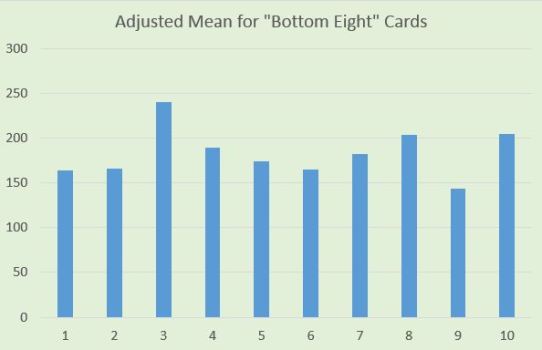
A better, though still imperfect, approach would aim for comparing apples to apples. One way of counteracting the inflation caused by Ruth, Gehrig, and other top stars is to restrict focus to common players only. Rather than agonize over player-by-player decisions as to who qualifies as common, the approach I’ll take is to consider only the bottom eight (based on population) players from each sheet.

Interestingly, the bar for Sheet 3 remains taller than all the other bars. However, there are changes to other bars on the graph. The Sheet 6 bar had been second tallest and is now just middle of the pack. The bars for the first two sheets also move closer together.
As a quick aside, Anson Whaley’s June 2018 post on Pre-War Cards noted the very different population reports for the set’s two Lou Gehrig cards. Specifically, the population numbers for the Sheet 6 Gehrig are much lower than those of the Sheet 3 Gehrig. Our latest graph provides at least a partial explanation.
Corroborating the data
There is always a danger in this sort of analysis that some key variable has been overlooked. At the risk of getting too silly, let’s pretend that a Tony Piet (sheet 9) super-collector were hoarding Piet cards and either keeping them raw or submitting to SGC or Beckett rather than PSA. At least potentially this could explain why our Sheet 9 bar is smaller than the others.
While there are several checks we can apply, the simplest is to see how the data in the above graph tracks with whichever player has the lowest population from each sheet. If we see the data as roughly parallel, we can feel pretty good about our data. Conversely, if we see poor tracking, that could be a sign that either some other force is at work or the data are just “too random” to work from.
This new graph appears to support the former, namely that averaging the bottom eight populations on each sheet does not seem to be impacted significantly by any outlier at the very bottom.

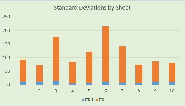
Another reassurance that the new data are fairly stable comes from looking at standard deviations. The spread of population data for a given sheet (orange bars) is very high while the spread among the lowest eight population cards (blue bars) is near zero. To put it slightly less technically, the bottom eight cards in a sheet all tell the same story.
Results so far
Were we to halt the analysis here, we would draw the following conclusions, at least to the degree that we trusted the methodology–
- Sheet 3 appears to have the highest production run, nearly 50% larger than many of the other sheets.
- Sheet 9 appears to have the smallest production run, roughly 10-20% scarcer than most of the other sheets.
- Sheets 1, 2, and 6 are nearly equal, as are Sheets 4, 5, and 7, and Sheets 8 and 10.
Still, I would caution rushing off to eBay to stock up on Sheet 9 commons just yet. There is at least one reason to believe the data are lying to us.
Monkey wrench from Sheet 6
I mentioned at the beginning that Sheet 6 is the one with the double-printed Babe Ruth card. Before jumping in to the monkey wrench, I’ll begin with the question of whether we should expect the population report for that Ruth to be twice as high as other cards in the sheet.
Focusing strictly on production runs, yes, there would have been twice as many Ruth 144 cards as, for example, Ray Kolp from that same sheet. If Goudey printed Sheet 6 three million times then we should expect they would have printed three million Ray Kolps and six million Ruth 144 cards.
However, two factors prevent such a ratio from surviving into the PSA population reports.
- More than likely, the Ruth cards survived at a higher rate than the Kolp cards.
- Definitely, collectors grade (and even regrade!) Ruth cards more than Kolp cards.
Based on these two factors, it should be no surprise the the ratio of Ruth 144 cards to Kolp cards is not 2:1 but 5:1. (The actual numbers are 1045 and 201.)
However, Sheet 6 doesn’t just have the double-printed Ruth 144. It also has the Ruth 149 (red) card. Should we not expect a 2:1 ratio in comparing Ruth to himself?

In fact, the ratio is more like 4:3. (Actual numbers are 1045 and 787. This should feel like a surprising result and possibly present enough of a monkey wrench as to regard the population reports as meaningless indicators of scarcity. Armed with this information, there are three main paths forward.
- Give up.
- Trust the numbers in spite of the Ruth anomaly.
- Introduce a new variable.
I’ll delve into the second of these a bit further as I think it’s less crazy than it sounds. Collectors back then weren’t thinking Babe Ruth cards were going to put their kids through college. These cards were fun to collect but essentially novelties rather than commodities.
Think back to the last worthless thing you ever collected. Maybe you were aiming to get the complete set of Snapple bottle caps. In my case, my son and I trolled the shores of Lake Superior for as many different kinds of rocks as we could find. As a kid, I collected cancelled stamps. In such cases, what would you do if you ended up with a duplicate, as would have happened a lot with Ruth 144? I know it sounds like heresy today, but you might well throw it away, whether right away or eventually.
(I’ll pause to indicate that this is a somewhat testable hypothesis, but we’ll save its pursuit for a bit later.)
A new variable
To get the math on the table before applying it to the cards, consider the numbers 13 and 9, which are clearly not in a 2:1 ratio. Now subtract 5 from each of them to get 8 and 4, which are in a 2:1 ratio. Now that you’ve survived the math, you’re probably wondering what it has to do with Babe Ruth.
There are 122 collectors on the PSA set registry for 1933 Goudey. Assume that these collectors (and 122 just like them but not on the registry) were motivated to chase down and grade one of each Ruth but had no need to double up on Ruth 144. The effect would be that the population of Ruth 144 cards would be underrepresented relative to its true number.
Our previous population numbers for Ruth 144 and Ruth 149 were 1045 and 787. If we adjust for the collectors–real and hypothetical–just described, the numbers become 801 and 543. What was once a 4:3 ratio becomes nearly 3:2. (In case you’re wondering we would have had to subtract away 529 such collectors to arrive at a 2:1 ratio.)
I am not ready to subtract away 529 or even 244, but I do believe that even if twice as many Ruth 144 cards as Ruth 149 cards somehow had survived into 2019 we should expect to see less than the full 2:1 ratio hit the population report. Though it’s an awesome card, the collectors out there who buy or submit graded Ruth cards would not be motivated to buy/submit this Ruth at twice the rate of the other Ruth cards in the set.
Back to throwing away doubles
Now that the “new variable” idea didn’t fully explain away the Ruth 144 anomaly, it’s worth returning to the idea that collectors in 1933 would have been less likely to retain doubles than singles. I mentioned this is at least partially a testable hypothesis, so let’s pursue it.
While the Ruth 144 card would have been the largest source of true doubles for collectors, there are two other card pairs that would have given less fastidious collectors near doubles. Lou Gehrig and Jimmie Foxx each have two cards in the set that are identical to each other aside from numbering.
If it was common practice to toss duplicates, we might expect the later-sheet cards of each of these three players to be more scarce than can be explained simply by the relative scarcity of the sheets. Here are the results.
For the Gehrig pair, the relevant sheets are 3 and 6. As inferred from the “bottom eight” population averages, we should expect there to be 72% as many Sheet 6 Gehrig cards as Sheet 3 Gehrig cards. Instead there are 57%, a drop-off of 15%.
For the Foxx pair, the relevant sheets are 1 and 6. As inferred from the “bottom eight” population averages, we should expect there to be the same number of Sheet 6 Foxx cards as Sheet 3 Foxx cards. Instead there are 78%, a drop-off of 22%.
Recalling again that the Gehrig and Foxx pairs are only near-duplicates whereas the double-printed Ruth 144 would have produced true duplicates, it’s reasonable to think the 15% and 22% discrepancies for Gehrig and Foxx could have been even higher for Ruth, as cringe-worthy as it is to picture anyone throwing his cards in the trash.
Back in business?
The 4:3 ratio of Ruth 144 to Ruth 149 cards (as opposed to 2:1) called into question the value of the PSA population data in understanding relative scarcity. However, the two approaches outline above (new variable, discard of duplicates) have the potential to explain away much or all of the gap. As such, I do believe the relative scarcity of the sheets as shown in the “bottom eight” graph is at least reasonably accurate.
So yes, we’re back in business. There are only two minor adjustments I believe apply.
Adjustment 1 – Set collectors
Imagine an alternate reality where the only cards submitted to PSA were from set registry collectors. Then regardless of the true distribution of cards in the wild, the PSA population data would tend to look fairly uniform. Meanwhile, in an alternate reality where there were no set collectors, we would expect the population data for common players to largely mirror their largely non-uniform distribution in the wild.
While those are both alternate realities, our true reality is not completely different. It’s simply a mixing of the two. The more we can remove the set collector data from the population data, the truer a picture we get of the cards overall.
I mentioned earlier that there are 122 registry collectors. About 40 have complete sets or near-complete sets. Though I regard the “bottom eight” graph as good enough, particularly if the only interest is in knowing which sheets are scarcer than others, I believe we come even closer to reality by subtracting 40 from each of the bars.
As all that happened was that each bar shrunk by 40, there are no changes to the ordering of the bars or even the height differences from bar to bar. However, the ratios from bar to bar do change.
Taking the Gehrig sheets as an example, the original “bottom eight” graph suggested the Sheet 6 production run was about 73% the size of Sheet 3. The revised graph puts this number at 68%. The difference is not a game-changer by any means, though it does help explain the actual pop differences on the two Gehrigs even more than before.
Adjustment 2 – Original collectors
This last adjustment is immaterial if the primary interest is in the relative scarcity of the Goudey cards today. It is also unsatisfying if you’re hoping for a newer, more accurate graph. Rather, it’s merely an observation that the data we’re sitting on right now remains an incomplete proxy for the original production runs.
As is the case with most very old baseball cards, the overwhelming majority of Goudey cards produced and sold in 1933 are no longer with us. Whether moms threw them out, kids themselves threw them out, or the dog ate them, the cards that remain are the exceptions and not the rule. In thinking about the cards that made it all the way from 1933 to the present, I imagine something of an 80-20 rule. Perhaps 80% of the cards came from the 20% of collectors who were really, really into collecting this set. Regardless of true variations in production runs, I expect such collectors would go the extra mile in chasing down or trading for the tougher cards and end up with collections looking at least a little more uniform than luck of the draw.
If so, then just as the first adjustment accentuated the differences among the sheets, this second adjustment would accentuate them even more. I will not even hazard a guess on just how much, but I’ll close by saying I believe the differences shown in our last graph reflect true differences today but understate the actual differences as they existed in 1933.
So what should I buy?
As always, the cards you want! But in case you’re wondering what the implications are for the megastars in the set, here is what my analysis implies:
The Sheet 9 cards appear to come from the smallest production run. Top cards from that sheet include these stunning cards of Grove, Dean, Hubbell, and Gehringer, along with Chuck Klein, Lefty Gomez, and Arky Vaughan.

Next on the list would be cards from Sheets 1, 2, and (most of) 6. Highlights of Sheet 1 include Jimmie Foxx’s card 29, Frank Frisch, Tony Lazzeri, Paul Waner, and Al Simmons. Sheet 2 superstars include Pie Traynor, Bill Dickey, and Bill Terry’s card 20. And finally, Sheet 6 superstars in this category include Ruth’s card 149, Gehrig’s card 160, Foxx’s card 154, and–if you like–Moe Berg. Ruth’s card 144 is omitted since its double-printing gives it the highest production in the entire set.
After that, five of the sheets are more or less middle of the pack, and only Sheet 3 stands out for (probably) having the highest production run. If scarce is what you’re after, then avoid paying top dollar for Eddie Collins, Lefty O’Doul’s card 58, Joe Cronin’s card 63, Lou Gehrig’s card 92, and Mickey Cochrane.
Finally, as mentioned already, the least rare card in the set is the one many collectors also believe is the set’s iconic card, the Ruth 144. (Kind of like 1989 Upper Deck!)
Obviously there’s a lot here to disagree with, but I hope there is at least some useful information for collectors hoping to better understand the 1933 Goudey set. And if you’d like to go beyond relative scarcity to absolute production numbers, head over to this next post.
